《Handbook of MRI Pulse Sequences》原著:MATT A. BERNSTEIN, KEVIN F. KING, XIAOHONG JOE ZHOU,SSFP-FID and SSFP-Echo SSFP-FID is a standard gradient-echo pulse sequence that provides greater signal than spoiled pulse sequences, but often at the cost of reduced contrast (Figure 14.4). It goes by a variety of commercial names (e.g., FISP) that are listed in Table 14.1. SSFP-echo is a less widely used pulse sequence, but is conceptually important for understanding the transverse steady state.SSFP-FID 与 SSFP-Echo
SSFP-FID 序列是标准的梯度回波序列,它的信号强度高于扰相梯度回波序列,但经常是以牺牲图像对比为代价(图 14.4)。它也被冠以各种商业名称(比如 FISP),见表 14.1。SSFP-echo 序列使用不太广泛,但它对于从概念上理解横向磁化矢量的稳态具有重要帮助。If the RF excitation pulses in the θ-TR-θ-TR-θ-TR... sequence are phase coherent and TR is less than or on the order of T2, then an SSFP (Carr 1958; Ernst and Anderson 1966) is established. In this context, phase coherent means that the RF pulses all have the same phase in the rotating frame, (i.e., θx-TR-θx-TR-θx...) or else a simple phase cycle such as sign alternation (θx-TR-θ(-x)-TR-θx-TR-θ(-x)-...). A further condition to avoid spoiling the steady state is that the phase accumulated by the transverse magnetization be the same in each TR interval. This condition requires that the gradient area in each TR interval be the same, so, for example, a phase-encoding rewinder lobe must be applied.
在序列 θ-TR-θ-TR-θ-TR... 中,如果射频激发脉冲的相位一致且 TR 小于 T2 量级或与 T2 量级相当,那么稳态自由进动 steady-state free precession SSFP(Carr 1958; Ernst and Anderson 1966)就建立了。此处,相位一致表示所有射频脉冲在旋转坐标系中拥有相同的相位(即 θx-TR-θx-TR-θx...),或拥有一简单的相位周期,比如正负交替(θx-TR-θ(-x)-TR-θx-TR-θ(-x)-...)。进一步避免稳态的扰乱就是在每个 TR 间期内横向磁化矢量累积的相位保持一致。那么这就需要每个 TR 间期内梯度的面积保持一致,例如,必须施加相位卷绕梯度。
TR is less than or on the order of T2要想获得横向磁化矢量的稳态,那么 TR 不能太长,太长的话,横向磁化矢量消散了,就不能被后续的 RF 进行回聚了,此也为一种扰相的方法(前面有提过)。那么为了不让横向磁化矢量消散,TR 必须要与 T2 保持一个量级,或者比 T2 的量级还要短。换句话说,就是如果组织的 T2 值约 100ms,那么 TR 也要是 100ms 左右,或者小于 100ms,比如 10ms、20ms 等。另外,每一个 RF,在梯度回波序列中,0<θ<90°,同样具有 0°、90° 与 180° 的效能。90° 效能将部分横向磁化矢量转变成纵向,以影响 SSFP-FID(引入 T2 对比),而 180° 效能产生 SSFP-Echo。
另外,如果射频脉冲的相位不一致的话,那么只能使得简单的正负相位交替方法,如果使用太多的不同的 RF 相位,那么就成了射频扰相了。
If these conditions are met, steady states for both the longitudinal magnetization and transverse magnetization will be established. The resulting SSFP of the transverse magnetization is schematically shown in Figure 14.7. It comprises two parts: an FID-like signal that forms just after each RF pulse and a time-reversed FID-like signal that forms just before each pulse. The former is called S+ or SSFP-FID, and the latter is called S- or SSFP-echo. If RF pulses are sign alternated, the amplitudes of the SSFP signals are unchanged, but their signs are reversed in every other TR interval, as shown in Figure 14.7b.如果这些条件都满足,那么纵向磁化矢量与横向磁化矢量都将达到稳态。产生的横向磁化矢量的稳态 SSFP 如图 14.7 所示,SSFP 由两部分组成:一个是类 FID 的信号,在每个 RF 脉冲激发后产生;另一个是时间反转的类 FID 信号,在每个 RF 脉冲激发前产生产生。前者称为 S+ 或 SSFP-FID,后者称为 S- or SSFP-echo。如果射频脉冲的符号(/极性)不断交替,那么 SSFP 信号的强度不变,但在每隔一个 TR 间期符号(/极性)变化一次,如图 14.7b 所示。

To calculate the strength of the SSFP-FID and SSFP-echo signals for GRE imaging, a two-step procedure is usually followed. (An alternative procedure is described in Gyngell 1988.) First, a recursion relation is set up that equates the magnetization in adjacent TR intervals, similar to Eq. (14.6). The procedure is more complicated than that used to derive Eq. (14.7), however, because both the transverse and longitudinal magnetization must be considered. Also, if sign alternation is used in the train of RF pulses, then the equality is assumed for every other TR interval. Details of the calculation are provided in Freeman and Hill (1971). Also a new parameter Φ is introduced, which is the angle through which the transverse magnetization precesses during each TR interval. The second step is to recognize that in GRE the imaging gradients introduce a spread of Φ across the voxel and to account for this spread by convolution (Zur et al. 1988). The final results of the calculation are presented in Hanicke and Vogel (2003):为了计算梯度回波成像的 SSFP-FID 和 SSFP-echo 信号强度,通常需要两个步骤。(还有另一种方法,见 Gyngell 1988。)首先,建立递推关系,并使得相邻两 TR 间期的磁化矢量相等,类似方程(14.6)。然而这一推导过程要比推导方程(14.7)的过程复杂很多,因为横向磁化矢量与纵向磁化矢量都要考虑进来。另外,如果射频脉冲使用的是极性交替的方案,那么要间隔 TR 建立等式关系。详细的推导计算过程可以参考 Freeman and Hill (1971)。同时还引入了一个新的参数 Φ,它是每个 TR 间期横向磁化矢量进动的相位角。第二步,认识到在梯度回波成像中,成像梯度在体素内引入了相位 Φ 的分布,对于这样的相位分布可以通过卷积来说明(Zur et al. 1988)。最终计算的结果见 in Hanicke and Vogel (2003):
The two lines in Eq. (14.15) are derived under the assumption that the SSFP-FID and SSFP-echo signals do not overlap substantially in the readout window. 方程(14.15)中两条式子成立的前提是假设 SSFP-FID 与 SSFP-echo 在信号读出时没有太多的重叠。
Also note that, from Eq. (14.16), an alternative algebraic form can be derived:并且注意到,从方程(14.16)可以推得另一种代数形式:

%%%%%%%%%%%%%%%
【译者注2】


%%%%%%%%%%%%%%%
Although the SSFP signal formulas in Eq. (14.15) are more complicated than the spoiled case in Eq. (14.8), there are some simple limiting cases. For example, if TR ≫ T2, then E2 is negligible, and
 and
and
 . Therefore
 , and with the aid of the trigonometric identity tan(u/2) = sinu/(1 + cosu):尽管方程(14.15)给出的 SSFP 信号强度公式比扰相梯度回波信号强度公式方程(14.8)复杂得多,但仍有一些简单的极限情况。例如,当 TR ≫ T2 时,E2 可以忽略不计,并且 、。那么
  ,并使用三角恒等式 tan(u/2) = sinu/(1 + cosu) 得:
%%%%%%%%%%%%%%%
【译者注3】

%%%%%%%%%%%%%%%
Equation (14.18) is the same as the expression for the spoiled case (Eq. 14.8), up to a factor of
 . If the SSFP-FID is rephased as a GRE at time TE, the two expressions become identical. This limiting case indicates that prolonging the TR and waiting for the transverse magnetization to decay away is an effective spoiling method.
方程(14.18)与方程(14.8)所表述的扰相梯度回波的情形是一样的,只相差个因子。如果在 SSFP-FID 在 TE 时刻使用梯度重聚采集梯度回波,那么这两个表述将完全相同。这一极限情况表明,延长 TR 时间使得横向磁化矢量消散是一种很好的扰相方法。
Another instructive case is
 , that is, the small flip angle limit. After some algebra, we find that
 . This in turn implies that:另一个具有意义的极限情况是当 时,也就是小翻转角的极限。经过一些代数运算我们有 , 那么:

that is the SSFP-FID becomes proton-density weighted at small flip angles, just like the spoiled signal in Eq. (14.8). 也就是 SSFP-FID 信号在小角度时变成了质子密度加权,就跟方程(14.8)所给的扰相梯度回波的极限情形一样。
%%%%%%%%%%%%%%%
【译者注4】


%%%%%%%%%%%%%%%
Despite the similarities between these two limiting cases, SSFP-FID and spoiled signals usually display substantially different contrast behavior. At intermediate and high flip angles, spoiled GRE provides considerable T1-weighting and dark fluid, whereas SSFP-FID provides less contrast but bright fluid (Figure 14.4). It is useful to remember that at fixed acquisition parameters (TR, TE, flip angle, etc.) the signal from SSFP-FID is greater than the signal from spoiled GRE. In other words, spoiled GRE obtains increased contrast by removing signal, mostly from tissue with a long T2, whereas SSFP-FID reuses transverse magnetization to increase signal.尽管在这两种极限情况中,SSFP-FID 与扰相梯度回波十分相似,但 SSFP-FID 与扰相梯度回波信号在对比度方面通常表现出很大的差异。当使用中等和较大翻角时,扰相梯度回波提供了相当大的 T1 权重,以及液体低信号;然而 SSFP-FID 得到的对比较差且液体为高信号(如图 14.4)。需要记住的是,当采集参数(TR, TE, 翻转角等)固定相同时,SSFP-FID 比扰相梯度回波信号强度高。换句话说,就是扰相梯度回波通过去除大多数来源于长 T2 组织的信号来提升对比;而 SSFP-FID 重复利用横向磁化矢量来提升信号强度。
The SSFP-echo signal can provide greater T2-weighting compared to the SSFP-FID, especially at intermediate and high flip angles. Simplifying the algebra by setting θ = 90° so that cosθ = 0 and using Eqs. (14.15) and (14.17), we find the ratio of the two signals is:
相较于 SSFP-FID,SSFP-echo 可以提供更多的 T2 权重,尤其是使用中等和较大的翻转角时。通过设定 θ = 90°(那么 cosθ = 0)而简化代数运算,并且利用方程 (14.15)与(14.17),我们得到两信号的比为:

Using Eq. (14.20) and the expansion
 ,the interested reader can show that in the case of TR ≪ T1, as
 :利用方程(14.20)与展开式 ,感兴趣的读者可以计算当 TR ≪ T1,即 时:

%%%%%%%%%%%%%%%
【译者注5】

%%%%%%%%%%%%%%%
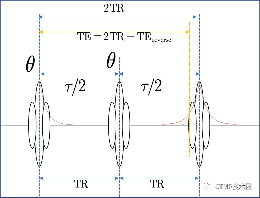
A physical interpretation of Eq. (14.21) is that the SSFP-echo signal is primarily composed of the SSFP-FID signal refocused from the previous TR interval, that is, TE = 2 × TR. If the echo is shifted to the left by an amount Δ to form a GRE as shown in Figure 14.11 (later in the chapter), then Eq. (14.21) is modified to
对于方程(14.12)的一个物理解释为,SSFP-echo 信号主要由 SSFP-FID 信号在前一个 TR 间期回聚产生的回波组成,也就是说,TE = 2 × TR。如果回波向左移 Δ 时间进行信号的采集,如图 14.11(在后面章节中),那么方程(14.21)需要做如下修正:


%%%%%%%%%%%%%%%
【译者注6】


%%%%%%%%%%%%%%%


 京公网安备 11010802020745号
工商备案公示信息
互联网药品信息服务资格证书((京)-非经营性-2020-0015)
京公网安备 11010802020745号
工商备案公示信息
互联网药品信息服务资格证书((京)-非经营性-2020-0015)


 010-82736610
 股票代码: 872612


