【Handbook of MRI Pulse Sequences】14.1.1 一连串射频脉冲后的磁化矢量响应

一切权利归原作者所有。

仅供学习交流使用，严禁用作商业用途。

Book：

《Handbook of MRI Pulse Sequences》

原著：MATT A. BERNSTEIN, KEVIN F. KING, XIAOHONG JOE ZHOU,

译注：蒋强盛

14.1.1 Response to A Series of RF Excitation Pulses

14.1.1 一连串射频脉冲后的磁化矢量响应

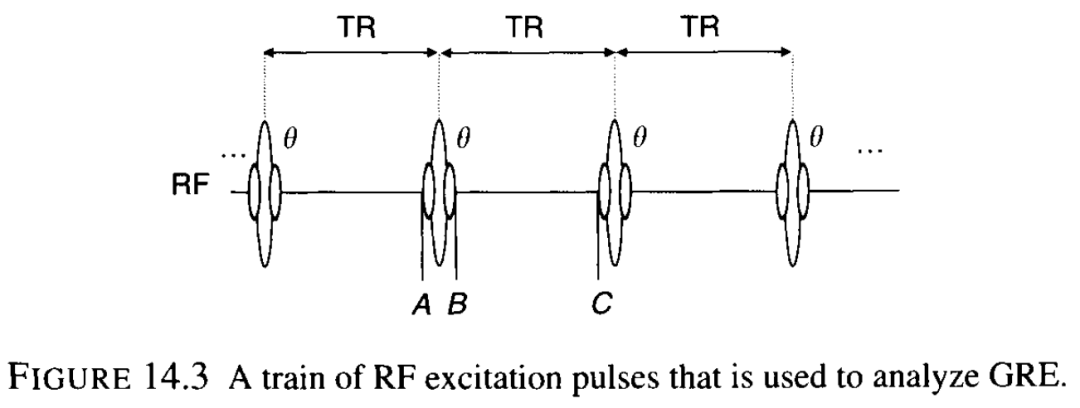
The excitation pulse is the only RF pulse in each TR interval, unless the GRE pulse sequence contains other modules (e.g., spatial saturation, magnetization transfer, spatial tagging, and magnetization preparation) that are described in other sections of the book. Even when some of those other modules are applied, they only affect selected magnetization (e.g., a spatial saturation band), so most of the magnetization in the imaging slice does not experience them. (An exception occurs for the MP-RAGE pulse sequence described in Section 14.2.) Therefore, much (if not all) of the magnetization in the imaging slice experiences a series of identical excitation pulses with flip angle θ, evenly spaced in time by TR (Figure 14.3). We assume that θ ≠ 0, ±180°, .... This θ-TR-θ-TR-θ-TR... pulse sequence is the basis used to analyze GRE. (Note that many authors label the flip angle of the excitation pulse in a GRE pulse sequence by the Greek letter α and refer to the excitation pulses as alpha-pulses. To be consistent with the other sections of the book, however, we continue to use the symbol θ.)

梯度回波序列的每个 TR 间期内只有激励脉冲是射频脉冲，除非包含其他模块（例如：空间饱和、磁化传递、空间标记和磁化准备）。包含其他模块的梯度回波序列在本书其他章节中将会讲述。即使当这些模块中的一些程序施加了，它们也仅只影响选择了的磁化矢量（比如空间饱和带），因此成像层面内的大多数其他磁化矢量并不受它们影响。（其中一个例外是 14.2 节中讲述的磁化准备快速梯度回波序列）因此，成像层面内的多数（如果不是全部的话）磁化矢量经受一连串完全相同的翻转角为 θ 的激励脉冲，它们以 TR 时间均匀分布（见图 14.3）。在这里，我们假设 θ ≠ 0, ±180°, ...。这一 θ-TR-θ-TR-θ-TR... 脉冲序列是分析梯度回波的基础。（另外，许多作者在标记梯度回波序列激励脉冲的翻转角时使用希腊字母 α ，并称此激励脉冲为 α-脉冲。然而，为了与此书其他章节保持一致，我们仍然使用字母 θ 来作为梯度回波序列的脉冲标记。）

The steady state is a concept that is repeatedly used in the study of gradient echoes. The steady state is also called dynamic equilibrium. If a system is not changing, and all of its parameters are constant, then the system is said to be in static equilibrium. A system that is continually changing can reach a steady state if the conditions are right. For example, if a bucket of water leaks but is being filled at exactly the same rate, the water level reaches a steady state. In GRE imaging, we consider steady states of both the longitudinal and transverse magnetization.

稳态这一概念在研究梯度回波时一直会用到。稳态又叫动态平衡。如果一个系统没有变化，并且所有参数恒定，那么这一系统被称作处于静态平衡。如果一系统一直变化且条件合适，那么能够达到一稳态。例如，如果一桶水一直漏水，但同时以相同的流速注入水，那么水位达到一稳态。在梯度回波成像中，我们讨论的稳态包括纵向稳态与横向稳态。

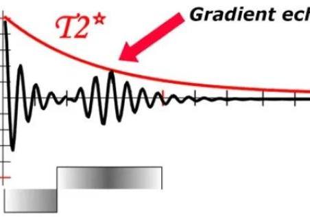
After a sufficient number of excitation pulses are applied, the longitudinal magnetization Mz reaches a steady state in GRE pulse sequences. That means that if we compare corresponding time points in adjacent TR intervals, the values of longitudinal magnetization Mz will be equal. GRE pulse sequences can be classified by the response of the transverse magnetization, M⊥. If M⊥ can be assumed to be zero just before each excitation pulse, then the GRE pulse sequence is said to be spoiled. If, however, the transverse magnetization reaches a (nonzero) steady state just before the application of each excitation pulse, then the pulse sequence is said to produce steady-state free precession (SSFP). The word free is used in the same sense as in free induction decay.

在梯度回波脉冲序列中，经过足够的射频脉冲激励后，纵向磁化矢量达到一稳态。也就是说，如果我们比较相邻 TR 间隙的相对应时间点，纵向磁化矢量  Mz 将相等。梯度回波序列可以通过横向磁化矢量 M⊥ 的响应情况来进行分类。如果在下一个激励脉冲到达前可以认为横向磁化矢量为零的话，那么这一梯度回波脉冲序列被称作被扰相的。然而，如果在下一个激励脉冲发射前，横向磁化矢量达到一（非零）稳态，那么称此脉冲序产生稳态自由进动（SSFP）。这里的自由与自由感应衰减中的自由一个意思。

Spoiling    Spoiled GRE pulse sequences can produce images with some T1-weighted contrast (Figure 14.4). These sequences go by a variety of names including spoiled Fast Low-Angle Shot (FLASH), spoiled gradient echo (SPGR), and T1 fast field echo (T1-FFE), as listed in Table 14.1. 

扰相    扰相梯度回波序列能够产生带有一定 T1 权重对比的图像（图 14.4）。这些序列被冠以各种各样的名字，其中包括扰相快速小角度激发（FLASH），扰相梯度回波（SPGR）和 T1 快速场回波（T1-FFE），如表 14.1 所列。

Spoiling can be accomplished in a variety of ways. The simplest method is to select TR that is at least four to five times T2, so that the transverse magnetization decays nearly to zero by the end of the pulse sequence. Because the main advantage of using GRE is acquisition speed, this is not a very practical spoiling method, unless the interleaved multislice acquisition strategy is used to increase the number of slice locations per TR (Section 11.5). For 2D sequential or 3D volume acquisitions, however, a different spoiling strategy must be used. End-of-sequence gradient spoiler (Section 10.5) pulses can be applied, but they are not effective at spoiling the transverse steady state unless their gradient area varies from TR to TR interval. Even with time-varying spoilers, the spoiling will be spatially nonuniform because gradients produce spatially varying fields. This is illustrated by the stripe pattern in Figure 14.5, which is obtained by using the phase-encoding gradient as a spoiler, (i.e., no phase rewinding lobe is used). A better solution is to use RF spoiling (Crawley et al. 1988; Zur et al. 1991; Duyn et al. 1997) to phase cycle the RF excitation pulses according to a predetermined schedule. RF spoiling not only provides more spatially uniform results, but also avoids eddy currents that vary among the TR intervals. Several RF phase-cycling schemes that produce good results are described in the literature.

扰相梯度回波可以通过多种方法实现。最简单的方法是选择长 TR，至少是 T2 弛豫时间的 4-5 倍，使得在下一个射频脉冲激发前横向磁化矢量衰减至接近零。因为使用梯度回波的主要优势是采集速度，那么这并不是一个非常实用的扰相方法，除非交叉多层采集时为了增加每个 TR 扫描的层数（第 11.5 节）而使用。然而，对于 2D 顺序采集或 3D 容积采集，必须使用不同的扰相方法。可以在信号采集完施加扰相梯度脉冲，但它对于横向磁化矢量稳态的扰相并不十分有效，除非每个 TR 扰相梯度的面积不同。即使使用了时变的扰相梯度，扰相在空间上也是不均匀的，因为梯度产生的是空间变化的磁场。那么就会产生条带伪影，如图 14.5，它使用相位编码梯度作为扰相梯度（即不施加相位卷绕梯度）。还有一个更好的扰相方案，就是使用射频扰相（Crawley et al. 1988; Zur et al. 1991; Duyn et al. 1997），按照预先设定好的来调整射频脉冲的相位，使得射频脉冲的相位呈现周期变化。射频扰相不仅能够提供空间更均匀的扰相结果，还能够避免每次扰相梯度施加时所产生的涡电流。在文献中，有好几个射频相位循环的方案可以得到良好的扰相结果。

Let Φj be the phase of the B1 field for the jth RF pulse in the rotating frame; Φ = 0 for a θx pulse, and Φ = 90° for θy. One method is to use randomized phases Φj, but then the effectiveness of the spoiling can fluctuate from TR to TR interval. A more popular method is to use a phase-cycling schedule such as:

令 Φj 是第 j 个射频脉冲 B1 场在旋转坐标系中的相位; θx 脉冲的 Φ = 0, θy 脉冲的 Φ = 90°。其中一种方法是使用随机相位 Φj, 但每个 TR 所达到的扰相效果不稳定。更流行的方法是使用相位循环方法，例如：

so that the phases Φ0, Φ1 = 2Φ0, Φ2 = 4Φ0, Φ3 = 7Φ0, ..., are applied. The starting value Φ0 is an adjustable parameter. The value Φ0 = 117 ° is recommended in Zur, Wood, and Neuringer (1991). Because the phase increment (Φj - Φj-1) in Eq. (14.2) is linearly proportional to j, the phase Φj varies quadratically with j. This quadratic dependence can be seen explicitly by solving the difference equation (14.2):

因此射频脉冲施加的相位顺序为 Φ0, Φ1 = 2Φ0, Φ2 = 4Φ0, Φ3 = 7Φ0, ...。起始相位值 Φ0 是一可调整的值。在文献 Zur, Wood, and Neuringer (1991) 中，推荐 Φ0 = 117 °。因为在方程（14.2）中，相位增量 (Φj - Φj-1) 与 j 呈线性关系，相位 Φj 与 j 呈二次关系。这一二次关系可以通过求解上述的差分方程（14.2）而清晰地得到：

%%%%%%%%%%%%%%%

【译者注1】

↑↑ from MRI from Picture to Proton, 3rd editon

%%%%%%%%%%%%%%%

With RF spoiling, the degree of spoiling depends strongly on the choice of Φ0, but unlike random phase methods it is uniform among the TR intervals. Note that RF-spoiled GRE pulse sequences must apply a phase-encoding rewinder because the gradient area on any of the three logical axes must not vary from TR to TR interval or else the spoiling will be spatially dependent. Also, during each TR interval, the received MR signal must be shifted by a phase Φj, so that the k-space data are consistent.

使用射频扰相，扰相的程度十分依赖于 Φ0 的选择，但不同于随机相位方法，这一方法中射频的相位是均匀分布的。需要注意的是，射频扰相梯度回波脉冲序列必须施加相位编码卷绕梯度，因为每个 TR 内三个逻辑轴上的梯度面积必须要保持一致，要不然扰相就具有空间依赖性。另外，在每个 TR 间期，采集接收到的 MR 信号必须经过 Φj 角度的相移，这样 k 空间数据才能保持一致。

Examining the structure of the stripes in Figure 14.5 can provide physical insight into RF spoiling and the choice of Φ0. The linear increment of the phase represented by Eq. (14.2) is equivalent to the phase twist imparted by the phase-encoding gradient as it is stepped to Fourier-encode an image. Because images such as Figure 14.5 are obtained using the phase-encoding gradient as a spoiler, they have the remarkable property of providing a spatial map of the effect of many different values of Φ0 between +180° and -180° in a single image. The bright stripes are unspoiled regions, corresponding to short phase cycles, such as Φ0 = 360°/n where n is a small integer. A phase advance of 360° is equivalent to Φ0 = 0°, or n = 1 (i.e., no phase cycling) and corresponds to the bright stripe in the center. A value of n = 2 (Φ0 = 180°) corresponds to negating every other pair of pulses; that is, it sets up a short phase cycle (of length 4 × TR) and produces the second brightest stripe, which is partially visible at the edge of the image. The dark regions are spoiled and correspond to phase cycles that have length much greater than T2/TR. This explains why a phase increment of 117° works well—no small integer multiple of 117° is divisible by 360°. Many other values of Φ0 (e.g., 123°) also produce good RF spoiling. Also note that the pattern of stripes is symmetric with respect to the center; that is, choosing a phase increment of -Φ0 produces the same effect as +Φ0.

仔细查看图 14.5 中的条带伪影结构，能够提供从物理角度来观察射频扰相和 Φ0 的选择问题。方程（14.2）中显示的相位的线性增量与傅立叶成像所使用的以固定大小相位编码梯度步级来施加相位编码梯度等效 。由于使用相位编码梯度作为扰相梯度，比如图 14.5，表现出了射频扰相使用不同的 Φ0 值（+180° ~ -180° ）而产生空间条带伪影的特性。白色条带表示未被扰相的区域，对应短的相位周期，比如 Φ0 = 360°/n，n 为一较小整数。相位差为 360° 等效于 Φ0 = 0°，或 n = 1（即没有相位循环）并且对应图像中心的白色条带。n = 2 (Φ0 = 180°)，即每隔一对脉冲产生一个相位周期；也就是，建立起短的相位周期（4 个 TR 长度）并且产生第二条白色条带，在图像的边缘可以看见，不是很明显。黑色区域表示被扰相的区域，并对应于很长的相位周期，远远大于 T2/TR。这也解释了为什么 117° 的相位增量表现得很好——360° 除以 117°  不能得到一个较小的整数。许多其他 Φ0 值（比如 123°）也能得到不错的射频扰相效果。另外注意到，条带的形式关于中心是对称的；也就是说，选择 -Φ0 的相位增量与 +Φ0 相位增量的效果是一样的。 

%%%%%%%%%%%%%%%

【译者注2】

The linear increment of the phase represented by Eq. (14.2) is equivalent to the phase twist imparted by the phase-encoding gradient as it is stepped to Fourier-encode an image.

相继的两个 RF 有固定的相位之差：

相继的两条相位编码线也有固定的相位编码梯度强度差别（固定的 ky 相位差别）。那么通过相位编码梯度的扰相就类似 RF 的相位之差。